Chapter 3 Probability introduction
3.1 Introduction to Probability
In this book, probability and statistics topics will be discussed extensively. Mainly the Bayesian interpretation of probability and Bayesian statistics. But we first need an intuitive conceptual basis to build on top of that. This chapter will build the foundations of probability theory, so we will assume minimal knowledge on the field and start from the basics.
Probability is a mathematical field that aims to measure the uncertainty of a particular event happening or the degree of confidence about some statement or hypothesis. As any other mathematical field, probability has its own axioms and definitions, and we will start learning them as we work through this chapter. An important feature of probability is how related it is to real world problems. The most fruitful probabilities fields are the ones that approach this kind of problem. You can see them being used in almost every scientific discipline.
Therefore, a nice way to introduce some of these concepts is by means of an experiment. Without further ado, let’s get started.
3.2 Events, sample spaces and sample points
Let’s make our first experiment. Consider a box with four balls inside of it, each one of these of a different color: blue, red, green and white.
#This libraries are just for uploading images into the Pluto notebook
begin
    using Images
    using ImageTransformations
    using Plots
endplot(imresize(load("./03_probability_intro/images/box-experiment.jpg"), (336, 400)),axis=nothing,border=:none)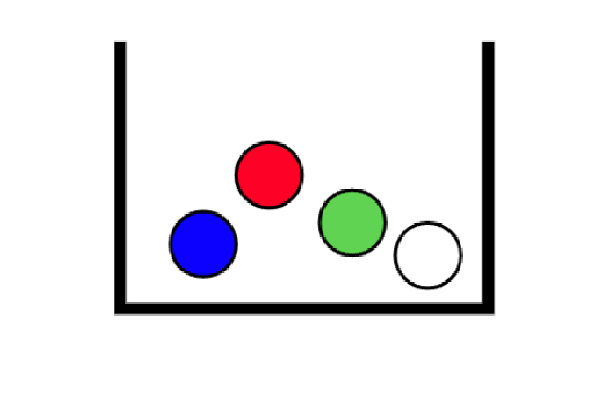
The experiment goes like this: We put our hands inside the box and take two balls at random, at the same time, and write down their colors. For example, red and green. We will refer to this outcome as \((R,G)\).
The possible outputs of our experiment are:
- Red Green = \((R,G)\)
- Red Blue = \((R,B)\)
- Red White = \((R,W)\)
- Green Blue = \((G,B)\)
- Green White = \((G,W)\)
- Blue White = \((B,W)\)
Notice that, since we don’t care about the orden in which the balls are taken out, saying “Red and Green” is equal to “Green and Red.”
To establish some terminology, we will define each possible output of the experiment as a sample point or simply a sample, and sample space as the aggregate of all the possible outcomes of an experiment.
In our example, the sample space will consist of a total of 6 sample points. This sample space can be thought schematically as a set containing all the possible sample points:
Sample space = \(\{(R,G), (R,B), (R,W), (G,B), (G,W), (B,W)\}\)
Suppose we wanted to know all the cases in which the white ball was taken out. This could be described as a subset of the sample space, the ones with the color white as one of the outcomes.
“The white ball was taken” = \(\{(R,W), (G,W), (B,W)\}\)
These subsets of the sample space are called events. There are as many events as possible subsets of the sample space, and they define everything we can expect from a given experiment. They can be expressed in colloquial language, as we can see in the example above; the event ‘The white ball was taken,’ corresponds to the subset \({(R,W), (G,W), (B,W)}\). This is so because the three sample points have a white ball among their constituent colors, and they represent all the possible realizations of our experiment that make our event true. We use capital letters to denote events
Other possible events associated with our experiment are,
A = “The red wall was not taken” = \(\{(G,B)(G,W)(B,W)\}\)
B = “The green and the blue ball were taken” = \(\{(G,B)\}\)
3.2.1 Relation among events
Events and the relationship between them can be represented using Venn diagrams. These are used widely in set theory, and since we are developing our probabilistic intuition thinking about possible outcomes as sets, they come in handy in this process.
Back to our experiment, the sample space consisted of:
Sample space = S = \(\{(R,G), (R,B), (R,W), (G,B), (G,W), (B,W)\}\)
Consider these two events,
A = “The white ball was taken” = \(\{(R,W), (G,W), (B,W)\}\)
B = “The red wall was not taken” = \(\{(G,B)(G,W)(B,W)\}\)
plot(imresize(load("./03_probability_intro/images/venn-1.jpg"), (336, 400)) ,axis=nothing,border=:none)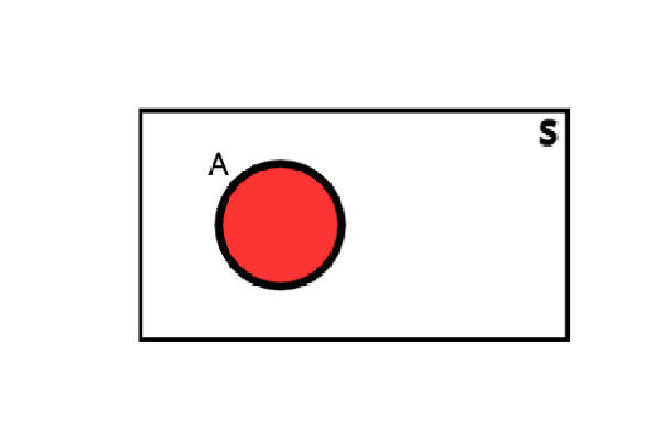
The rectangle represents the sample space S. Since it represents all the possible outputs of our experiment, nothing can be outside it.
Then we represent the event A, that contains the 3 sample points \(\{(R,W), (G,W)\) and \((B,W)\}\), with a red circle.
The event consisting of all points not contained in the event A is defined as the complementary event (or negation) of A and is denoted by A’.
\(A´= {(R,G),(R,B),(G,B)}\)
Notice that if we created a new event that contains all the sample points of A and A´, we would have obtained the sample space.
plot(imresize(load("./03_probability_intro/images/venn-3.jpg"), (336, 400)) ,axis=nothing,border=:none)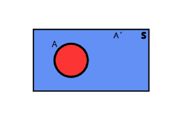
Now let’s take into account the event B. The points \((G,W)\) and \((B,W)\) are both present in the events A and B, so we must represent them in this way:
plot(imresize(load("./03_probability_intro/images/venn-2.jpg"), (336, 400)) ,axis=nothing,border=:none)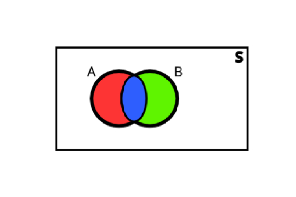
The blue area contains the sample points that are in both events, in this case \((G,W)\) and \((B,W)\). It is defined as the intersection of A and B and is denoted by \(A \cap B\).
On the other hand, the red area contains the points that are only present in the event A, in this case \((R,W)\) . Analogously, the green area contains the points that are only present in the event A, in this case \((G,B)\) .
3.3 Probability
Now that we have introduced the event, sample point and sample space concepts, we can start talking about probability.
Probability is a measure of our belief that a particular event will occur, and we express it with a number ranging from \(0\) to \(1\). The number \(0\) means we have the strongest possible belief that the event will not happen: We are sure it will not happen. The number \(1\) means we have the strongest possible belief that the event will happen: We are sure it will happen. Probability, being a measure of our own belief or certainty in the occurrence of an event, does not determine whether the event occurs or not. For this reason, events may still occur when we assign them probability \(0\), and they might not occur if we assign them probability \(1\).
By definition, the probability of the entire sample space \(S\) is unity, or \(P\{S\} = 1\). It follows that for any event \(A: 0 <P(A) <1\).
In our experiment we can consider that all the sample points have the same realization probability, so we assign \(\frac{1}{6}\) to each one. Of course, this is an assumption we make, considering that no ball has some distinctive property and that they are distributed randomly in the box. For example, if one of the balls had a rugged surface, the equal probabilities assumption would not hold. But let’s keep it simple
Since we consider that all the sample points have the same realization probability, another way we can assign probabilities to each one is with the popular formula:
\(P(A) = \frac{success \ cases} {total \ cases}\)
\(P((R,W))= \frac{(R,W)}{(R,G),(R,B),(R,W),(G,B),(G,W),(B,W)} =\frac{1}{6}\)
The probability \(P(A)\) of any event \(A\) is the sum of the probabilities of each of the sample points in it.
For A = “The white ball was taken” = \(\{(R,W), (G,W), (B,W)\}\)
\(P(A) = P(R,W) + P(G,W)+ P(B,W) = \frac{1}{6}+ \frac{1}{6} + \frac{1}{6} = \frac{3}{6} = 0.5\)
\(P(A´) = P(R,G) + P(R,B) + P(G,B) = \frac{1}{6}+ \frac{1}{6} + \frac{1}{6} = 0.5\)
B= “The red wall was not taken” = \(\{(G,B)(G,W)(B,W)\}\)
\(P(B) = \frac{3}{6}\)
\(A \cap B = \{(G,W),(B,W)\)
\(P(A \cap B) = \frac{2}{6}\)
For any two events A and B the probability that either A or B or both occur is given by
\(P(A \cup B) = P(A) + P(B) - P(A \cap B)\)
\(P(A \cup B) =\frac{3}{6} + \frac{3}{6} - \frac{1}{6}= \frac{5}{6}\)
Another example:
\(P(A \cup A´)= P(A) + P(A´) - P(A \cap A´) = \frac{3}{6} + \frac{3}{6} - 0= 1\)
3.4 Conditional probability
The notion of conditional probability is a basic tool of probability theory.
Given two events A and B, the conditional probability of A given B, is noted as \(P(A|B)\). Similarly, the conditional probability of B given A is noted as \(P(B|A)\). In general, these two probabilities need not to be equal. The way to interpret \(P(A|B)\) is: ‘the probability of the event A happening, given that we know the event B occurred.’ The analogous interpretation for \(P(B|A)\) would be ‘the probability of event B happening, given that we know the event A occurred.’ Although it may sound as if this implies an order in the occurrence of the events, that isn’t necessarily the case. What in reality has an actual order in this statement is our knowledge of what things happened. If we say, for example \(P(A|B)\), then what we know first is event B, and given this knowledge, we want to know the probability of event A.
To see it in a visual way:
plot(imresize(load("./03_probability_intro/images/venn-4.jpg"), (336, 400)) ,axis=nothing,border=:none)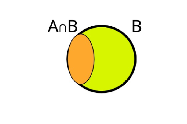
Notice that, since we know B occurred we can truncate the sample space to the B event, and now calculate the probability of A.
\(P(A|B) = \frac{P(A \cap B)}{P(B)}\)
Consider these two events,
A = “I pick a red and a green ball”
B = “I pick a red ball”
P(A|B) is interpreted as the probability of picking a red and a green ball knowing that I already picked one red ball.
\(A = \{(R,G),(R,B),(R,W)\} => P(A) = \frac{3}{6}\)
\(B = \{(R,G)\} => P(B) => \frac{3}{6}\)
\(A \cap B = \{(R,G)\} => P(A \cap B) = \frac{1}{6}\)
\(P(A|B) = \frac{P(A \cap B)}{P(B)}\)
\(P(A|B) = \frac{1}{6} ÷ \frac{3}{6} = \frac{1}{3}\)
Now, let’s conclude our experiment and delve into more interesting problems.
3.5 Joint probability
We refer to joint probability as the probability of two events occurring together and at the same time. For two general events A and B, their joint probability is denoted:
\(P(A\text{ and }B)\)
Let’s see how it works with an example.
Imagine we want to calculate the probability of these two events occurring together and at the same time, denoted :\(P(L\text{ and }R)\)
R = “Today It will rain”
L = “The number 39 will win the lottery”
To calculate the joint probability of these two events, we use the formula,
\(P(A\text{ and }B) = P(A)P(B|A)\)
For the events R and L:
\(P(R\text{ and }L) = P(R)P(L|R)\)
Let’s analyze the nature of these events a little bit, are they related? Technically, we can think everything in our planet is interconnected with everything else, but in practice, it is fair to assume these two events are pretty independent from one another. In a more formal way, what this is telling us is that knowing the probability of one of the events does not give us information about the probability of the other event. That is the definition of independence in this context.
In the language of probabilities, we can write a special property for independent events.
\(P(R|L) = P(R) \text{ either } P(L|R) = P(L)\)
replacing in the joint probability formula,
\(P(R\text{ and }L) = P(R) * P(L)\)
Colloquially, this means that the probability of both events “Today It will rain” and “The number 39 will win the lottery” happening together is equal to the product of each of the probabilities of each one happening individually.
Now, lets study the joint probability of this two not independent events:
R = “Today It will rain”
H = “humidity will exceed 50%”
If it is raining, there is a high probability that the humidity levels will rise, so it is natural to think about these events as dependent.
To calculate the joint probability:
\(P(H\text{ and }R) = P(R)P(H|R)\)
In a more general way, for two arbitrary events A and B,
\(P(A\text{ and }B) = P(A)P(B|A)\)
With this formula in mind, and another property of conjunction probability,
\(P(A\text{ and }B) = P(B\text{ and }A)\)
which just means what we naturally interpret of two events happening at the same time. If the two events do happen at the same time, it doesn’t matter if we write \(B\text{ and }A)\) or \(A\text{ and }B\), setting an order in the expression is just a consequence of having to write it. Just like doing \(2 + 3\) or \(3 + 2\), the ‘and’ logical operator is commutative.
3.6 Bayes theorem
With this concepts in mind we will now proceed to derive the famous Bayes’ theorem.
\(P(B\text{ and }A) = P(B)P(A|B)\)
And putting all the pieces together,
\(P(B)P(A|B) = P(A)P(B|A) \implies P(A|B) = \frac{P(A)P(B|A)}{P(B)}\)
Summing up, we arrived to Bayes’ theorem:
\(P(A|B) = \frac{P(A)P(B|A)}{P(B)}\)
This theorem does not only give us a practical way to calculate conditional probabilities, but also is the fundamental building block of the Bayesian interpretation of probability. But what does this even mean? Here we must take a step back and focus on the details of how exactly probability is defined for an event or hypothesis.
There are two main approaches to probability, the frequentist approach and the one we have already introduced, the Bayesian one. The frequentist interpretation views probability as the frequency of events when a big number of repetitions are carried out. The typical example of this is the flipping of a coin. To know the probability of obtaining heads when flipping a coin, a frequentist will tell you to perform an experiment with a lot of coin tosses (say, 1000 repetitions). You write down the outcome (heads or tails) of each flip and then you calculate the heads ratio over the total amount of repetitions, i.e.: \(P(H) = 511 / 1000 = 0,511\). This will be your probability from a pure frequentist point of view.
The Bayesian point of view has a more general interpretation. It is not bound to the frequency of events. Probability is thought as a degree of uncertainty about the event happening and also takes into account our current state of knowledge about that event. In a Bayesian way of thinking one could assign (and actually it is done extensively) a probability to events such as the election of some politician, while in the frequentist view this would make no sense, since we can’t make large repetitions of the election to know the frequency underlying that event.
You might be asking yourself: How does this Bayesian probability work? What is the hidden mechanism inside of it? Take another look at Bayes’ theorem. We have talked about it applying to events and hypotheses. To really get a grasp of the meaning behind the Baseyian interpretation of probability, we should think about some hypothesis \(H\) and some data \(D\) we are interested in to check the validity of our hypothesis. In this view, Bayes’ theorem is written as
\(P(H|D) = \frac{P(D|H)P(H)}{P(D)}\)
Put into words, what this means is ‘the probability of my hypothesis or belief, given the data observed, is equal to the probability that the data would be obtained if the belief were to be true, multiplied by the probability of the hypothesis being true before seeing the data, divided by the probability of obtaining that data.’ This may sound a bit confusing at first, but if you look closely for some time and think about each term, you will find it makes perfect sense.
P(H): This is called Prior probability. As its name states, it represents the probability of a particular belief or hypothesis of being true before we have any new data to contrast this belief.
P(D|H): Frequently called Likelihood. If we remember the definition of conditional probability, what this means is the probability of the data being observed if our hypothesis were true. Intuitively, if we collect some data that contradicts our beliefs, this probability should be low. Makes sense, right?
P(D): This term has no particular name. It is a measure of all possible ways we could have obtained the data be have. In general it is considered a normalizing constant.
P(H|D): The famous Posterior probability. Again, remembering the definition of conditional probability, it is clear this represents the probability of our hypothesis being true, given that we collected some data \(D\).
It is interesting to give a little more detail on the epistemological interpretation of this entire theorem. We start from some initial hypothesis and we assign some probability to it (the Prior). How exactly this has to be done is uncertain, in fact, there are ways to encode that you don’t know anything about the validity of the hypothesis. But the important part is that, if you already knew something about it, you can include that in your priors. For example, if you are trying to estimate some parameter that you know is positive definite, then you can use priors that are defined only for positive values. From that starting point, then, you have a methodical way to update your beliefs by collecting data, and with this data, give rise to the Posterior probability, which hopefully will be more accurate than our Prior probability. What is nice about the Bayesian framework is that we always account for the uncertainty of the world. We start with some probability and end with another probability, but uncertainty is always present. This is what real life is about. To understand the full power of Bayesian probability we have to extend the notion of probability to probability density. We will discuss this topic in the following section.
3.7 Probability distributions
So far, we have been talking of probabilities of particular events. Probability distributions, on the other hand, help us compute probabilities of various events. We can distinguish between discrete and continuous cases depending on the possible output of the experiment.
3.7.1 Discrete Case
If the outputs of our experiment are discrete, then the probability distribution is called a probability mass function, where we assign a probability to each possible outcome.
One of the most popular distributions is the Poisson distribution. Suppose I want to visualize the probability of receiving x spam mails on Mondays.
begin
    using Distributions
    using StatsPlots

    bar(Poisson(1.5), xlabel="Spam emails", ylabel="Probability", legend=false, size=(400, 300))
end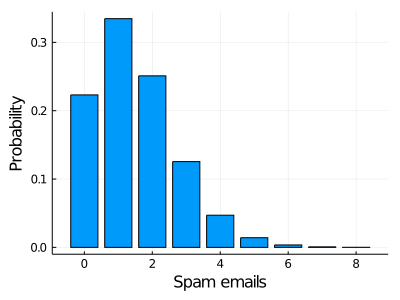
Here we represent the probability of receiving x spam mail in a day. The interpretation of this graph is pretty straightforward. The probability of receiving 0 spam emails on a Monday is approximately 0.2, for 1 spam email is slightly higher than 0.3 and so on, we have the probability of each possible output.
λ=4bar(Poisson(λ), xlabel="x", ylabel="Probability", legend=false, size=(400, 300))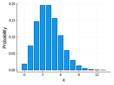
3.7.2 Continuous cases
Instead of a probability mass function, a continuous variable has a probability density function.
For example, consider the density probability of heights of adult women, given approximately by a Normal distribution,
begin
    plot(Normal(64, 3), xlabel="Height (in)", ylabel="Probability density", legend=false, size=(400, 300))
end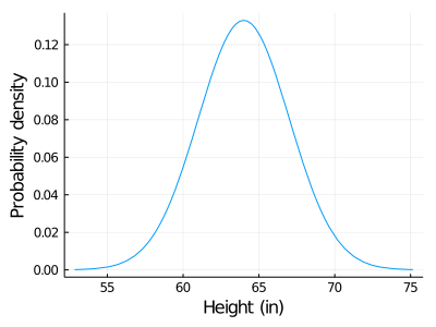
In this example, the event space is just all the possible heights a woman could have, in other words, the x axis. The y axis, on the other hand, represents the probability density.
To not delve into complex definitions, we can think of the x label as a steel bar and the y label the density of each infinitesimal point of the bar. If we want to know the mass of a specific segment we need to calculate the area below the curve of that segment (integrate the segment mathematically talking). Since we are using the probability density, instead of the mass what we obtain is the probability.
When we work with continuous variables it is pointless to talk about the probability of a single x value. Think of it in a mathematical way, in a number line there are infinity points in between 0 and 0,01. In this case, our continuous variable is women’s height, since there are infinitely possible heights it has no sense to talk about the probability of a single height, like \(P(6 in)\).
Probability in the continuous case is always computed in an interval. For example, suppose we want to know the probability that a randomly selected woman measures between 60 and 65 inches. To know it we need to calculate the area under the density curve in the intervals x = [60,65].
Keep in mind that the x label contains all possible events, in this case all possible women´s heights, so the area below the curve of all the x label is equal to 1.
An alternative description of the distribution is the cumulative distribution function also called the distribution function. It describes the probability that the random variable is no larger than a given value. We obtain it by integrating the density function and
plot(imresize(load("./03_probability_intro/images/density and cumulative functions.png"), (300, 860)),axis=nothing,border=:none)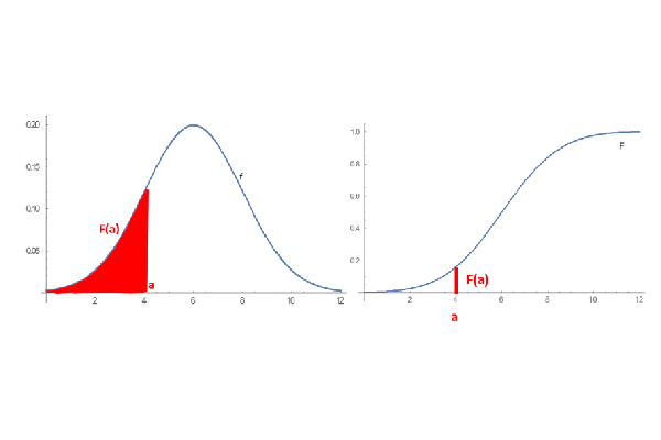
On the left is the probability density function and on the right is the cumulative distribution function, which is the area under the probability density curve.
Any mathematical function satisfying certain requirements can be a probability density. There are lots of these types of functions, and each one has its own shape and distinctive properties.
We will introduce some important probability density functions so that you can have a better understanding of what all this is about. Probably, the concept of the Normal distribution –also referred as the Gaussian– was already familiar to you, as it is one of the most popular and widely used distributions in some fields and in popular culture. The shape of this distribution is governed by two parameters, usually represented by the Greek letters \(\mu\) and \(\sigma\). Roughly speaking, \(\mu\) is associated with the center of the distribution and \(\sigma\) with how wide it is
μ = 0 σ= 2.5plot(Normal(μ,σ), xlabel="x", ylabel="P(x)", lw=4, color="purple", label=false, size=(450, 300), alpha=0.8, title="Normal distribution", xlim=(-10, 10))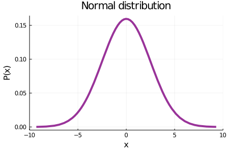
Every probability density that is defined by a mathematical function, has a set of parameters that defines the distribution’s shape and behaviour, and changing them will influence the distribution in different ways, depending on the one we are working with.
Another widely used distribution is the exponential. Below you can see how it looks. It is governed by only one parameter, \(\alpha\), which basically represents the rate of decrease in probability as \(x\) gets bigger.
One last slider to change the value of the \(α\) parameter of exponential distribution can be implemented if you replicate the code below.
α= 1.5plot(Exponential(α), xlabel="x", ylabel="P(x)", lw=4, color="blue", label=false, size=(450, 300), alpha=0.8, title="Exponential distribution", xlim=(0, 10))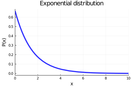
As the book progresses, we will be using a lot of different distributions. They are an important building block in probability and statistics. In the next section, we will discuss a little bit about how probability arises from gathering data.
3.7.3 Histograms
To illustrate some of these concepts we have been learning, we are going to use monthly rainfall data from the city of Buenos Aires, Argentina, since 1991. The histogram of the data is shown below. You may be wondering what a histogram is. An histogram is a plot that tells us the counts or relative frequencies of a given set of events.
As a data scientist you are constantly working with datasets and a great first approach to that dataset is by constructing a histogram. To construct a histogram, the first step is to bin the range of values that is, divide the entire range of values into a series of intervals and then count how many values fall into each interval
begin
    using CSV
    using DataFrames
    #Read the CSV file and transform it into a DataFrame
    rain_data = CSV.read("./03_probability_intro/data/historico_precipitaciones.csv", DataFrame)
    #Rename the columns
    colnames = ["Year", "Month", "mm", "Days"]
    rename!(rain_data, Symbol.(colnames)) #Symbol is the type of object used to represent the labels of a dataset

    #We use a dictionary to translate de Month names
    translate = Dict("Enero" => "January" ,"Febrero" => "February" ,"Marzo" => "March" ,"Abril" => "April" ,"Mayo" => "May" ,"Junio" => "June"  ,"Julio" => "July"   ,"Agosto" => "August"  ,"Septiembre" => "September"  ,"Octubre" => "October" ,"Noviembre" => "November" ,"Diciembre" => "December")

    for i in 1:length(rain_data[:,:Month])
        rain_data[i,:Month] = translate[rain_data[i,:Month]]
    end
end
We can see the first few rows of our data, with columns corresponding to the year, the month, the rain precipitation (in millimeters) and the number of days it rained in that month.
first(rain_data, 8)## 8×4 DataFrame
## Row │ Year Month mm Days
## │ Int64 String Float64 Int64
## ─────┼─────────────────────────────────
## 1 │ 1991 January 190.0 7
## 2 │ 1991 February 30.5 6
## 3 │ 1991 March 55.0 8
## 4 │ 1991 April 125.6 12
## 5 │ 1991 May 68.4 7
## 6 │ 1991 June 119.7 10
## 7 │ 1991 July 89.3 8
## 8 │ 1991 August 66.4 7Now plotting the histogram for the column of rainfall in mm we have the figure shown below. Plotting a histogram is very easy with the Plots.jl package. You just have to pass the array you want to make the histogram of and the number of bins. The other arguments are self-explanatory, and are just to make the plot nicer.
begin
    histogram(rain_data[:,"mm"], bins=20, legend=false, size=(450, 300))
    title!("Monthly rainfall in Buenos Aires")
    xlabel!("Rainfall (mm)")
    ylabel!("Frequency")
end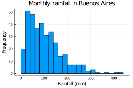
Histograms give us a good approximation of the probability density or mass function. The reason behind this is because we have registered some total number \(N\) of events that happened in some time interval (in this case, one month) and we grouped the number of times each one occurred. In this line of reasoning, events that happened most are more likely to happen, and hence we can say they have a higher probability associated with them. Something important to consider about histograms when dealing with a continuous variable such as, in our case, millimeters of monthly rainfall, are bins and bin size. When working with such continuous variables, the domain in which our data expresses itself (in this case, from 0 mm to approximately 450 mm) is divided in discrete intervals. In this way, given a bin size of 20mm, when constructing our histogram we have to ask ‘how many rainy days have given us a precipitation measurement between 100mm and 120mm?’ and then we register that number in that bin. This process is repeated for all bins to obtain our histogram.
We have earlier said that probability has to be a number between 0 and 1, so how can it be that these relative frequencies are linked to probabilities? What we should do now is to normalize our histogram to have the frequency values constrained. Normalizing is just the action of adjusting the scale of variables, without changing the relative values of our data. Below we show the normalized histogram. You will notice that the frequency values are very low now. The reason for this is that when normalizing, we impose to our histogram data that the sum of the counts of all our events (or, thinking graphically, the total area of the histogram) must be 1. But why? As probability tells us how plausible is an event, if we take into account all the events, we expect that the probability of all those events to be the maximum value, and that value is 1 by convention. When we normalize a histogram, we obtain another histogram that approaches the probability density function. So, we normalize the histogram obtaining:
begin
    histogram(rain_data[:,"mm"], bins=20, legend=false, normalize=true, size=(450, 300))
    title!("Monthly rainfall in Buenos Aires")
    xlabel!("Rainfall [mm]")
    ylabel!("Frequency")
end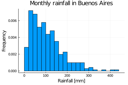
There is a lot we can say about this plot. First, it is worth noting that a rainfall amount less than \(0\)mm is not possible, that’s why we don’t have any event in this region. On the other hand, we see that a monthly rainfall higher than \(300\)mm is a rare event, and a rainfall higher than \(400\)mm is even less likely to happen.
But why am I inferring how likely is an event to happen in the future with data from the past?
I’m making some assumptions that are often implied working with histograms and measured data: the first assumption is that the data is representative for the variable in consideration, meaning that the data of rainfall was measured well, that it isn’t measured just during winter for example, when we know rainfall is most common. The other big assumption is that things in the future will not change much from things in the past, so if we do the measure again for some time in the near future, the shape of the histogram is going to be more or less the same. These assumptions may or may not hold in the real events, but this doesn’t mean there is something wrong with our analysis or how we model our data. It’s just that we chose some assumptions that seem reasonable with the information we have. And we always have to make some assumptions to obtain answers.
So far we have been talking about histograms as probability density functions. Distributions such as these, that are built from the outcome of an experiment are called empirical distributions. This means that they arise from direct measurements, not from an underlying analytical function. When dealing with most real-world examples, histograms will represent distributions we will obtain for our updated beliefs, so they are a really important concept for what will come in the book.
All the concepts we developed about probability density, are directly applied to our Bayesian formalism. The prior, likelihood and posterior probabilities are really probability densities, and that is really how we treat Bayes’ theorem mathematically and computationally.
3.8 Example: Bayesian Bandits
Now we are going to tackle a famous problem that may help us to understand a little bit how to incorporate what we learned about Bayesian probability and some features of the Julia language. Here we present the bandit or multi-armed bandit problem. Although it is conceived thinking about a strategy for a casino situation, there exist a lot of different settings where the same strategy could be applied.
The situation, in it’s simpler form, goes like this: you are in a casino, with a limited amount of casino chips. In front of you there are some slot machines (say, three of them for simplicity). Each machine has some probability \(p_m\) of giving you $1 associated with it, but every machine has a different probability. There are two main problems. First, we don’t know these probabilities beforehand, so we will have to develop some explorative process in order to gather information about the machines. The second problem is that our chips –and thus our possible trials– are limited, and we want to take the most profit we can out of the machines. How do we do this? Finding the machine with the highest success probability and keep playing on it. This tradeoff is commonly known as explore vs. exploit. If we had one million chips we could simply play a lot of times in each machine and thus make a good estimate about their probabilities, but our reward may not be very good, because we would have played so many chips in machines that were not our best option. Conversely, we may have found a machine which we know that has a good success probability, but if we don’t explore the other machines also, we won’t know if it is the best of our options.
This is a kind of problem that is very suited for the Bayesian way of thinking. We start with some information about the slot machines (in the worst case, we know nothing), and we will update our beliefs with the results of our trials. A methodology exists for these explore vs. exploit dilemmas, within many others, which is called Thompson sampling. The algorithm underlying the Thompson sampling can be thought in these successive steps:
- First, assign some probability distribution for your knowledge of the success probability of each slot machine.
- Sample randomly from each of these distributions and check which is the maximum sampled probability.
- Pull the arm of the machine corresponding to that maximum value.
- Update the probability with the result of the experiment.
- Repeat from step 2.
Here we will take some advantage about the math that can be used to model our situation. To model the generation of our data, we can use a distribution we have not yet introduced, the Binomial distribution. This distribution arises when you repeat some experiment that has two possible outcomes, a number N of times. In each individual experiment, the outcomes have some probability \(p\) and \(1-p\) of happening (because there are only two). Let’s see what this Binomial distribution looks like,
p = 0.5N = 250scatter(Binomial(N, p), xlim=300, label=false, title="Binomial distribution", size=(500, 350), xlabel="Number of succeses")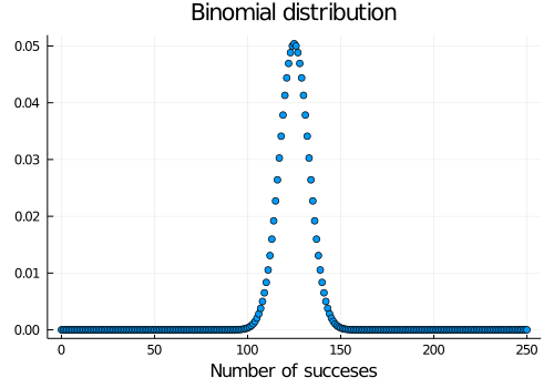
We choose this distribution as it models properly our situation, with \(p\) being the probability we estimate of succeeding with a particular machine, and \(N\) the number of trials we make on the machine. The two possible outcomes are success (we win $1) or fail (we don’t win anything)
So we now use a prior to set our knowledge before making a trial on the slot machine. The thing is, there exists a mathematical hack called conjugate priors. When a likelihood distribution is multiplied by its conjugate prior, the posterior distribution is the same as the prior with its corresponding parameters updated. This trick frees us from the need of using more computation-expensive techniques, that we will be using later in the book. In the particular case of the Binomial distribution, the conjugate prior is the Beta distribution. This is a very flexible distribution, as we can obtain a lot of other distributions as particular cases of the Beta, with specific combinations of its parameters. Below you can see some of the fancy shapes this Beta distribution can obtain
begin
    plot(Beta(1, 1), ylim=(0, 5), size=(400, 300), label=false, xlabel="x", ylabel="P(x)", title="Beta distribution shapes")
    plot!(Beta(0.5, 0.5), label=false)
    plot!(Beta(5, 5), label=false)
    plot!(Beta(10, 3), label=false)
    plot!(Beta(3, 10), label=false)
end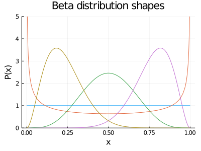
To start formalizing our problem a bit, we are going to start building our bandits. This is just a way to name our slot machines and some information associated with them. How will we do this? With the help of Julia’s struct. These are objects we can create in Julia and that can be used to store information that has meaning as an entire block. In our case, some relevant information would be to store the probability of each slot machine, and the number of trials. It is more comfortable to carry all this information in one big block, as we later can start creating as many bandits we want, and it would be impossible to keep track of all the parameters. Above we define a struct of a beta bandit, which will store the real probability of success of the bandit, the parameters \(a\) and \(b\) of the Beta distribution, and the total number of tries \(N\) of the bandit. This would correspond to the first step in the Thompson sampling algorithm.
begin
    mutable struct beta_bandit
        # the real success probability of the bandit
        p::Float64
        # a parameter from the beta distribution (successes)
        a::Int64
        # b parameter from the beta distribution (fails)
        b::Int64
        # total number of trials of bandit
        N::Int64
        # initialization of the Beta distribution with parameters a=1, b=1 (uniform distribution)
        beta_bandit(p=p, a=1, b=1, N=0) = new(p, a, b, N)
    end
end
Given that we have constructed our bandit and assigned a probability distribution to it, we define the function to sample from the distribution, as we will be needing it for the second step of the Thompson sampling algorithm.
sample_bandit(bandit::beta_bandit) = rand(Beta(bandit.a, bandit.b))## sample_bandit (generic function with 1 method)Now we need some function to pull an arm of the slot machine and actually test if we get a success or not. This will help us in the second step of the algorithm.
pull_arm(bandit::beta_bandit) = bandit.p > rand()## pull_arm (generic function with 1 method)Finally, we define another function to update the bandit information, based on the result of pulling an arm. This corresponds to the forth step in the Thompson sampling algorithm.
function update_bandit(bandit::beta_bandit, outcome::Bool)
    if outcome
        bandit.a += 1
    else
        bandit.b += 1
    end
    bandit.N += 1
end
## update_bandit (generic function with 1 method)With all these functions defined, we are ready to make an experiment and actually see how our strategy works. We will define beforehand a number of trials and the true probabilities of the slot machines. When the experiment is over, we will see how well were the probabilities of each machine were estimated, and the reward we accumulated. If you come up with some other novel strategy, you can test it doing a similar experiment and see how well the probabilities were estimated and the final reward you got. First, we define the total number of trials we are going to make, and then the true probabilities of each slot machine. At the end, we’ll see how well these probabilities were estimated, or, in other words, how well the Thompson sampling helped in the process of gathering information about the bandits.
N_TRIALS = 100## 100BANDIT_PROBABILITIES = [0.3, 0.5, 0.75]## 3-element Array{Float64,1}:
## 0.3
## 0.5
## 0.75function beta_bandit_experiment(band_probs, trials)
bandits = [beta_bandit(p) for p in band_probs]
reward = 0
for i in 1:trials
# _, mxidx = findmax([rand(Beta(bandit.a, bandit.b)) for bandit in bandits])
_, mxidx = findmax([sample_bandit(bandit) for bandit in bandits])
best_bandit = bandits[mxidx]
exp = pull_arm(best_bandit)
if exp
reward += 1
end
update_bandit(best_bandit, exp)
end
plot()
for i in 1:length(bandits)
display(plot!(Beta(bandits[i].a, bandits[i].b), xlim=(0, 1), lw=2, xlabel="Success probability of bandit", ylabel="Probability density"))
end
return reward, current()
end## beta_bandit_experiment (generic function with 1 method)rew, bandit_plot = beta_bandit_experiment(BANDIT_PROBABILITIES, N_TRIALS);bandit_plot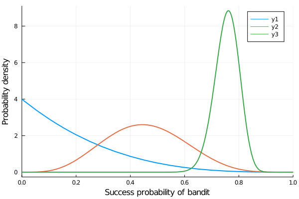
Considering that we have only tried 100 times, the probabilities have been estimated pretty well! Each distribution assigns a high-enough probability to the true value of the bandit probabilities and its surroundings. Other strategies rather than the Thompson sampling can be tested to see how well they perform, this was just a simple example to apply Bayesian probability.
3.9 Summary
In this chapter, we introduced the basic concepts of probability. We talked about the probability of independent events and about conditional probability, which led us to Bayes’ theorem.
Then, we addressed the two main approaches to probability: the frequentist approach and the Bayesian one, where our initial beliefs can be updated with the addition of new data. We also learned what a probability distribution is, we went over a few examples and saw why Bayesians use them to represent probability.
Finally, we saw the multi-armed bandit problem in which we have a limited amount of resources and must allocate them among competing alternatives to infer the one with the highest probability of success. To solve it, we constructed a Bayesian model using the Thompson sampling algorithm.
3.10 References
- Bayesian Statistics the fun way
- Infinite Powers: How Calculus Reveals the Secrets of the Universe
- Statistical Rethinking
- ThinkBayes
- ThinkStats
- Mixture Distribution
- A contextual bandit bake-off
- Bandit Algs page
- Bayesian Methods for Hackers
- An Introduction to Probability Theory and Its Applications, Vol. 1