Chapter 2 Meeting Julia
2.1 Why Julia
People have asked us why we wrote this book using Julia instead of Python or R, which are the current standards in the data science world. While Python and R are also great choices, Julia is an up and coming language that will surely have an impact in the coming years.
It performs faster than pure R and Python (as fast as C) while maintaining the same degree of readability, allowing us to write highly performant code in a simple way. Julia is already being used in many top-tier tech companies and scientific research —there are plenty of scientists and engineers of different disciplines collaborating with Julia, which gives us a wide range of possibilities to approach different problems. Often, libraries in languages like Python or R are optimized to be performant, but this usually involves writing code in other languages better suited for this task such as C or Fortran, as well as writing code to manage the communication between the high level language and the low level one. Julia, on the other hand, expands the possibilities of people who have concrete problems that involve a lot of computation. Libraries can be developed to be performant in plain Julia code, following some basic coding guidelines to get the most out of it. This enables useful libraries to be created by people without programming or Computer Science expertise.
2.2 Julia presentation
Julia is a free and open-source general-purpose language, designed and developed by Jeff Bezanson, Alan Edelman, Viral B. Shah and Stefan Karpinski at MIT. Julia is created from scratch to be both fast and easy to understand, even for people who are not programmers or computer scientists. It has abstraction capabilities of high-level languages, while also being really fast, as its slogan calls “Julia looks like Python, feels like Lisp, runs like Fortran.”
Before Julia, programming languages were limited to either having a simple syntax and good abstraction capabilities and therefore user-friendly or being high-performance, which was necessary to solve resource-intensive computations. This led applied scientists to face the task of not only learning two different languages, but also learning how to have them communicating with one another. This difficulty is called the two-language problem, which Julia creators aim to solve with this new language.
Julia is dynamically typed and great for interactive use. It also uses multiple dispatch as a core design concept, which adds to the composability of the language. In conventional, single-dispatched programming languages, when invoking a method, one of the arguments has a special treatment since it determines which of the methods contained in a function is going to be applied. Multiple dispatch is a generalization of this for all the arguments of the function, so the method applied is going to be the one that matches exactly the number of types of the function call.
2.3 Installation
For the installation process, we recommend you follow the instructions provided by the Julia team:
Platform Specific Instructions for Official Binaries: These instructions will get you through a fresh installation of Julia depending on the specifications of your computer. It is a bare bones installation, so it will only include the basic Julia packages.
All along the book, we are going to use specific Julia packages that you have to install before calling them in your code. Julia has a built-in packet manager that makes the task of installing new packages and checking compatibilities very easy. First, you will need to start a Julia session. For this, type in your terminal
~ julia
julia>
At this point, your Julia session will have started. What you see right now is a Julia REPL (read-eval-print loop), an interactive command line prompt. Here you can quickly evaluate Julia expressions, get help about different Julia functionalities and much more. The REPL has a set of different modes you can activate with different keybindings. The Julian mode is the default one, where you can directly type any Julia expression and press the Enter key to evaluate and print it. The help mode is activated with an interrogation sign ‘?’ . You will notice that the prompt will now change,
julia> ?
help?>
By typing the name of a function or a Julia package, you will get information about it as well as usage examples. Another available mode is the shell mode. This is just a way to input terminal commands in your Julia REPL. You can access this mode by typing a semicolon,
julia> ;
shell>
Maybe one of the most used, along with the default Julian mode, is the package manager mode. When in this mode, you can perform tasks such as adding and updating packages. It is also useful to manage project environments and controlling package versions. To switch to the package manager, type a closing square bracket ‘],’
julia> ]
(@v1.5) pkg>
If you see the word ‘pkg’ in the prompt, it means you accessed the package manager successfully. To add a new package, you just need to write
(@v1.5) pkg> add NewPackageIt is as simple as that! All Julia commands are case-sensitive, so be sure to write the package name –and in the future, all functions and variables too– correctly.
2.4 First steps into the Julia world
As with every programming language, it is useful to know some of the basic operations and functionalities. We encourage you to open a Julia session REPL and start experimenting with all the code written in this chapter to start developing an intuition about the things that make Julia code special.
The common arithmetical and logical operations are all available in Julia:
- \(+\): Add operator
- \(-\): Subtract operator
- \(*\): Product operator
- \(/\): Division operator
Julia code is intended to be very similar to math. So instead of doing something like
julia> 2*xyou can simply do
julia> 2xFor this same purpose, Julia has a great variety of unicode characters, which enable us to write things like Greek letters and subscripts/superscripts, making our code much more beautiful and easy to read in a mathematical form. In general, unicode characters are activated by using ‘\,’ followed by the name of the character and then pressing the ‘tab’ key. For example,
julia> \beta # and next we press tab
julia> β
You can add subscripts by using ‘_’ and superscripts by using ‘^,’ followed by the character(s) you want to modify and then pressing Tab. For example,
julia> L\_0 # and next we press tab
julia> L₀
Unicodes behave just like any other letter of your keyboard. You can use them inside strings or as variable names and assign them a value.
julia> β = 5
5

julia> "The ⌀ of the circle is $β "
"The ⌀ of the circle is 5 "
Some popular Greek letters already have their values assigned.
julia> \pi # and next we press tab
julia> π
π = 3.1415926535897...

julia> \euler # and next we press tab
julia> ℯ
ℯ = 2.7182818284590...
You can see all the unicodes supported by Julia here
The basic number types are also supported in Julia.
We can explore this with the function typeof(), which outputs the type of its argument, as it is represented in Julia.
Let’s see some examples,
julia>typeof(2)
Int64

julia>typeof(2.0)
Float64

julia>typeof(3 + 5im)
Complex{Int64}
These were examples of integers, floats and complex numbers. All data types in Julia start with a capital letter. Notice that if you want to do something like,
julia> 10/2
5.0
the output is a floating point number, although the two numbers in the operation are integers. This is because in Julia, division of integers always results in floats. When valid, you can always do
julia> Int64(5.0)
5
to convert from one data type to another.
Following with the basics, let’s take a look at how logical or boolean operations are done in Julia. Booleans are written as ‘true’ and ‘false.’ The most important boolean operations for our purposes are the following:
 !: \"not\" logical operator
 &: \"and\" logical operator
 |: \"or\" logical operator
 ==: \"equal to\" logical operator
 !=: \"different to\" logical operator
 >: \"greater than\" operator
 <: \"less than\" operator
 >=: \"greater or equal to\" operator
 <=: \"less or equal to\" operator
Some examples of these,
julia> true & true
true

julia> true & false
false

julia> true & !false
true

julia> 3 == 3
true

julia> 4 == 5
false

julia> 7 <= 7
true
Comparisons can be chained to have a simpler mathematical readability, like so:
julia> 10 <= 11 < 24
true

julia> 5 > 2 < 1
false
The next important topic in this Julia programming basics, is the strings data type and basic manipulations. As in many other programming languages, strings are created between ‘",’
julia> "This is a Julia string!"
"This is a Julia string!"
You can access a particular character of a string by writing the index of that character in the string between brackets right next to it. Likewise, you can access a substring by writing the first and the last index of the substring you want, separated by a colon, all this between brackets. This is called slicing, and it will be very useful later when working with arrays. Here’s an example:
julia> "This is a Julia string!"[1] # this will output the first character of the string and other related information.
'T': ASCII/Unicode U+0054 (category Lu: Letter, uppercase)

julia> "This is a Julia string!"[1:4] # this will output the substring obtained of going from the first index to the fourth
"This"
A really useful tool when using strings is string interpolation. This is a way to evaluate an expression inside a string and print it. This is usually done by writing a dollar symbol $ $ $ followed by the expression between parentheses. For example,
julia> "The product between 4 and 5 is $(4 * 5)"
"The product between 4 and 5 is 20"
This wouldn’t be a programming introduction if we didn’t include printing ‘Hello World!’
, right?
Printing in Julia is very easy.
There are two functions for printing: print() and println().
The former will print the string you pass in the argument, without creating a new line.
What this means is that, for example, if you are in a Julia REPL and you call the print() function two or more times, the printed strings will be concatenated in the same line, while successive calls to the println() function will print every new string in a new, separated line from the previous one.
So, to show this we will need to execute two print actions in one console line.
To execute multiple actions in one line you just need to separate them with a ;.
julia> print("Hello"); print(" world!")
Hello world!


julia> println("Hello"); println("world!")
Hello
world!
It’s time now to start introducing collections of data in Julia. We will start by talking about arrays. As in many other programming languages, arrays in Julia can be created by listing objects between square brackets separated by commas. For example,
julia> int_array = [1, 2, 3]
3-element Array{Int64,1}:
 1
 2
 3

julia> str_array = ["Hello", "World"]
2-element Array{String,1}:
 "Hello"
 "World"
As you can see, arrays can store any type of data. If all the data in the array is of the same type, it will be compiled as an array of that data type. You can see that in the pattern that the Julia REPL prints out:
Firstly, it displays how many elements there are in the collection. In our case, 3 elements in int_array and 2 elements in str_array. When dealing with higher dimensionality arrays, the shape will be informed.
Secondly, the output shows the type and dimensionality of the array. The first element inside the curly brackets specifies the type of every member of the array, if they are all the same. If this is not the case, type ‘Any’ will appear, meaning that the collection of objects inside the array is not homogeneous in its type.
Compilation of Julia code tends to be faster when arrays have a defined type, so it is recommended to use homogeneous types when possible.
The second element inside the curly braces tells us how many dimensions there arein the array. Our example shows two one-dimensional arrays, hence a 1 is printed. Later, we will introduce matrices and, naturally, a 2 will appear in this place instead a 1.
- Finally, the content of the array is printed in a columnar way.
When building Julia, the convention has been set so that it has column-major ordering. So you can think of standard one-dimensional arrays as column vectors, and in fact this will be mandatory when doing calculations between vectors or matrices.
A row vector (or a \(1\)x\(n\) array), in the other hand, can be defined using whitespaces instead of commas,
julia> [3 2 1 4]
1×4 Array{Int64,2}:
 3  2  1  4
In contrast to other languages, where matrices are expressed as ‘arrays of arrays,’ in Julia we write the numbers in succession separated by whitespaces, and we use a semicolon to indicate the end of the row, just like we saw in the example of a row vector. For example,
julia> [1 1 2; 4 1 0; 3 3 1]
3×3 Array{Int64,2}:
 1  1  2
 4  1  0
 3  3  1
The length and shape of arrays can be obtained using the length() and size() functions respectively.
julia> length([1, -1, 2, 0])
4

julia> size([1 0; 0 1])
(2, 2)

julia> size([1 0; 0 1], 2) # you can also specify the dimension where you want the shape to be computed
2
An interesting feature in Julia is broadcasting. Suppose you wanted to add the number 2 to every element of an array. You might be tempted to do
julia> 2 + [1, 1, 1]
ERROR: MethodError: no method matching +(::Array{Int64,1}, ::Int64)
For element-wise addition, use broadcasting with dot syntax: array .+ scalar
Closest candidates are:
  +(::Any, ::Any, ::Any, ::Any...) at operators.jl:538
  +(::Complex{Bool}, ::Real) at complex.jl:301
  +(::Missing, ::Number) at missing.jl:115
  ...
Stacktrace:
 [1] top-level scope at REPL[18]:1
As you can see, the expression returns an error. If you watch this error message closely, it gives you a good suggestion about what to do. If we now try writing a period ‘.’ right before the plus sign, we get
julia> 2 .+ [1, 1, 1]
3-element Array{Int64,1}:
 3
 3
 3
What we did was broadcast the sum operator ‘+’ over the entire array. This is done by adding a period before the operator we want to broadcast. In this way we can write complicated expressions in a much cleaner, simpler and compact way. This can be done with any of the operators we have already seen,
julia> 3 .> [2, 4, 5] # this will output a bit array with 0s as false and 1s as true
3-element BitArray{1}:
 1
 0
 0
If we do a broadcasting operation between two arrays with the same shape, whatever operation you are broadcasting will be done element-wise. For example,
julia> [7, 2, 1] .* [10, 4, 8]
3-element Array{Int64,1}:
 70
  8
  8

julia> [10 2 35] ./ [5 2 7]
1×3 Array{Float64,2}:
 2.0  1.0  5.0

julia> [5 2; 1 4] .- [2 1; 2 3]
2×2 Array{Int64,2}:
  3  1
 -1  1
If we use the broadcast operator between a column vector and a row vector instead, the broadcast is done for every row of the first vector and every column of the second vector, returning a matrix,
julia> [1, 0, 1] .+ [3 1 4]
3×3 Array{Int64,2}:
 4  2  5
 3  1  4
 4  2  5
Another useful tool when dealing with arrays are concatenations. Given two arrays, you can concatenate them horizontally or vertically. This is best seen in an example
julia> vcat([1, 2, 3], [4, 5, 6]) # this concatenates the two arrays vertically, giving us a new long array
6-element Array{Int64,1}:
 1
 2
 3
 4
 5
 6

julia> hcat([1, 2, 3], [4, 5, 6]) # this stacks the two arrays one next to the other, returning a matrix
3×2 Array{Int64,2}:
 1  4
 2  5
 3  6
With some of these basic tools to start getting your hands dirty in Julia, we can get going into some other functionalities like loops and function definitions.
We have already seen a for loop.
For loops are started with a for keyword, followed by the name of the iterator and the range of iterations we want our loop to cover.
Below this for statement we write what we want to be performed in each loop and we finish with an end keyword statement.
Let’s return to the example we made earlier,
julia> for i in 1:100
           println(i)
       end
The syntax 1:100 is the Julian way to define a range of all the numbers from 1 to 100, with a step of 1.
We could have set 1:2:100 if we wanted to jump between numbers with a step size of 2.
We can also iterate over collections of data, like arrays.
Consider the next block of code where we define an array and then iterate over it,
julia> arr = [1, 3, 2, 2]
julia> for element in arr
           println(element)
       end
1
3
2
2
As you can see, the loop was done for each element of the array. It might be convenient sometimes to iterate over a collection.
Conditional statements in Julia are very similar to most languages.
Essentially, a conditional statement starts with the if keyword, followed by the condition that must be evaluated to true or false, and then the body of the action to apply if the condition evaluates to true.
Then, optional elseif keywords may be used to check for additional conditions, and an optional else keyword at the end to execute a piece of code if all of the conditions above evaluate to false.
Finally, as usual in Julia, the conditional statement block finishes with an end keyword.
julia> x = 3
julia> if x > 2
           println("x is greater than 2")
       elseif 1 < x < 2
           println("x is in between 1 and 2")
       else
           println("x is less than 1")
       end
x is greater than 2
Now consider the code block below, where we define a function to calculate a certain number of steps of the Fibonacci sequence,
julia> n1 = 0
julia> n2 = 1
julia> m = 10
julia> function fibonacci(n1, n2, m)
           fib = Array{Int64,1}(undef, m)
           fib[1] = n1
           fib[2] = n2
           for i in 3:m
               fib[i] = fib[i-1] + fib[i-2]
           end
           return fib
       end
fibonacci (generic function with 1 method)
Here, we first made some variable assignments, variables \(n1\), \(n2\) and \(m\) were assigned values 0, 1 and 10.
Variables are assigned simply by writing the name of the variable followed by an ‘equal’ sign, and followed finally by the value you want to store in that variable.
There is no need to declare the data type of the value you are going to store.
Then, we defined the function body for the fibonacci series computation.
Function blocks start with the function keyword, followed by the name of the function and the arguments between brackets, all separated by commas.
In this function, the arguments will be the first two numbers of the sequence and the total length of the fibonacci sequence.
Inside the body of the function, everything is indented.
Although this is not strictly necessary for the code to run, it is a good practice to have from the bbeginning, since we want our code to be readable.
At first, we initialize an array of integers of one dimension and length \(m\), by allocating memory.
This way of initializing an array is not strictly necessary, you could have initialized an empty array and start filling it later in the code.
But it is definitely a good practice to learn for a situation like this, where we know how long our array is going to be and optimizing code performance in Julia.
The memory allocation for this array is done by initializing the array as we have already seen earlier.
julia {Int64,1}just means we want a one-dimensional array of integers.
The new part is the one between parenthesis, julia (undef, m).
This just means we are initializing the array with undefined values –which will be later modified by us–, and that there will be a number \(m\) of them.
Don’t worry too much if you don’t understand all this right now, though.
We then proceed to assign the two first elements of the sequence and calculate the rest with a for loop.
Finally, an end keyword is necessary at the end of the for loop and another one to end the definition of the function.
Evaluating our function in the variables \(n1\), \(n2\) and \(m\) already defined, gives us:
julia> fibonacci(n1, n2, m)
10-element Array{Int64,1}:
  0
  1
  1
  2
  3
  5
  8
 13
 21
 34
Remember the broadcasting operation, that dot we added to the bbeginning of another operator to apply it on an entire collection of objects? It turns out that this can be done with functions as well! Consider the following function,
julia> function isPositive(x)
          if x >= 0
               return true
          elseif x < 0
               return false
          end
       end
isPositive (generic function with 1 method)

julia> isPositive(3)
true

julia> isPositive.([-1, 1, 3, -5])
4-element BitArray{1}:
 0
 1
 1
 0
As you can see, we broadcasted the isPositive() function over every element of an array by adding a dot next to the end of the function name.
It is as easy as that!
Once you start using this feature, you will notice how useful it is.
One thing concerning functions in Julia is the ‘bang’(!) convention.
Functions that have a name ending with an exclamation mark (or bang), are functions that change their inputs in-place.
Consider the example of the pop!
function from the Julia Base package.
Watch closely what happens to the array over which we apply the function.
julia> arr = [1, 2, 3]
julia> n = pop!(arr)
3
julia> arr
2-element Array{Int64,1}:
 1
 2
julia> n
3
Did you understand what happened?
First, we defined an array.
Then, we applied the pop!() function, which returns the last element of the array and assigns it to n.
But notice that when we call our arr variable to see what it is storing, now the number 3 is gone.
This is what functions with a bang do and what we mean with modifying in-place.
Try to follow this convention whenever you define a function that will modify other objects in-place!
Sometimes, you will be in a situation where you may need to use some function, but you don’t really need to give it name and store it, because it’s not very relevant to your code.
For these kinds of situations, an anonymous or lambda function may be what you need.
Typically, anonymous functions will be used as arguments to higher-order functions.
This is just a fancy name to functions that accept other functions as arguments, that is what makes them of higher-order.
We can create an anonymous function and apply it to each element of a collection by using the map() keyword.
You can think of the map() function as a way to broadcast any function over a collection.
Anonymous functions are created using the arrow -> syntax.
At the left-hand side of the arrow, you must specify what the arguments of the function will be and their name.
At the right side of the arrow, you write the recipe of the things to do with these arguments.
Let’s use an anonymous function to define a not-anonymous function, just to illustrate the point.
julia> f = (x,y) -> x + y
#1 (generic function with 1 method)
julia> f(2,3)
5
You can think about what we did as if \(f\) were a variable that is storing some function.
Then, when calling \(f(2,3)\) Julia understands we want to evaluate the function it is storing with the values 2 and 3.
Let’s see now how the higher-order function map() uses anonymous functions.
We will broadcast our anonymous function x^2 + 5 over all the elements of an array.
julia> map(x -> x^2 + 5, [2, 4, 6, 3, 3])
5-element Array{Int64,1}:
  9
 21
 41
 14
 14
The first argument of the map function is another function. You can define new functions and then use them inside map, but with the help of anonymous functions you can simply create a throw-away function inside map’s arguments. This function we pass as an argument, is then applied to every member of the array we input as the second argument.
"""
Now let’s introduce another data collection: Dictionaries.
A dictionary is a collection of key-value pairs. You can think of them as arrays, but instead of being indexed by a sequence of numbers they are indexed by keys, each one linked to a value.
To create a dictionary we use the function Dict() with the key-value pairs as arguments.
Dict(key1 => value1, key2 => value2).
julia> Dict("A" => 1, "B" => 2)
Dict{String,Int64} with 2 entries:
  "B" => 2
  "A" => 1
So we created our first dictionary. Let’s review what the Julia REPL prints out:
Dict{String,Int64} tells us the dictionary data type that Julia automatically assigns to the pair (key,value).
In this example, the keys will be strings and the values, integers.
Finally, it prints all the (key => value) elements of the dictionary.
In Julia, the keys and values of a dictionary can be of any type.
julia> Dict("x" => 1.4, "y" => 5.3)
Dict{String,Float64} with 2 entries:
  "x" => 1.4
  "y" => 5.3

julia> Dict(1 => 10.0, 2 => 100.0)
Dict{Int64,Float64} with 2 entries:
  2 => 100.0
  1 => 10.0
Letting Julia automatically assign the data type can cause bugs or errors when adding new elements.
Thus, it is a good practice to assign the data type of the dictionary ourselves.
To do it, we just need to indicate it in between brackets { } after the Dict keyword:
Dict{key type, value type}(key1 => value1, key2 => value2)
julia> Dict{Int64,String}(1 => "Hello", 2 => "Wormd")
Dict{Int64,String} with 2 entries:
  2 => "Wormd"
  1 => "Hello"
Now let’s see the dictionary’s basic functions.
First, we will create a dictionary called “languages” that contains the names of programming languages as keys and their release year as values.
julia> languages = Dict{String,Int64}("Julia" => 2012, "Java" => 1995, "Python" => 1990)

Dict{String,Int64} with 3 entries:
  "Julia"  => 2012
  "Python" => 1990
  "Java"   => 1995
To grab a key’s value we need to indicate it in between brackets [].
julia> languages["Julia"]
2012
We can easily add an element to the dictionary.
julia> languages["C++"] = 1980
1980

julia> languages
Dict{String,Int64} with 4 entries:
  "Julia"  => 2012
  "Python" => 1990
  "Java"   => 1995
  "C++"    => 1980
We do something similar to modify a key’s value:
julia> languages["Python"] = 1991
1991

julia> languages
Dict{String,Int64} with 3 entries:
  "Julia"  => 2012
  "Python" => 1991
  "C++"    => 1980
Notice that the ways of adding and modifying a value are identical. That is because keys of a dictionary can never be repeated or modified. Since each key is unique, assigning a new value for a key overrides the previous one.
To delete an element we use the delete! method.
julia> delete!(languages,"Java")
Dict{String,Int64} with 3 entries:
  "Julia"  => 2012
  "Python" => 1990
  "C++"    => 1980
To finish, let’s see how to iterate over a dictionary.
julia> for(key,value) in languages
               println("$key was released in $value")
       end
Julia was released in 2012
Python was released in 1991
C++ was released in 1980
"""
Now that we have discussed the most important details of Julia’s syntax, let’s focus our attention on some of the packages in Julia’s ecosystem."
2.5 Julia’s Ecosystem: Basic plotting and manipulation of DataFrames
Julia’s ecosystem is composed by a variety of libraries which focus on technical domains such as Data Science (DataFrames.jl, CSV.jl, JSON.jl), Machine Learning (MLJ.jl, Flux.jl, Turing.jl) and Scientific Computing (DifferentialEquations.jl), as well as more general purpose programming (HTTP.jl, Dash.jl). We will now consider one of the libraries that will be accompanying us throughout the book to make visualizations, Plots.jl.
To install the Plots.jl library we need to go to the Julia package manager mode as we saw earlier.
julia> ]
(@v1.5) pkg>
(@v1.5) pkg> add Plots.jl
There are some other great packages like Gadfly.jl and VegaLite.jl, but Plots will be the best to get you started.
Let’s import the library with the ‘using’ keyword and start making some plots.
We will plot the first ten numbers of the fibonacci sequence using the scatter() function.
begin
    using Plots

    sequence = [0, 1, 1, 2, 3, 5, 8, 13, 21, 34]

    scatter(sequence, xlabel="n", ylabel="Fibonacci(n)", color="purple", label=false, size=(450, 300))
end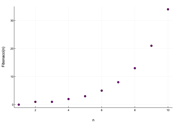
2.5.1 Plotting with Plots.jl
Let’s make a plot of the 10 first numbers in the fibonacci sequence.
For this, we can make use of the scatter() function:
The only really important argument of the scatter function in the example above is sequence, the first one, which tells the function what is the data we want to plot.
The other arguments are just details to make the visualization prettier.
Here we have used the scatter function because we want a discrete plot for our sequence.
In case we wanted a continuous one, we could have used plot().
Let’s see this applied to our fibonacci sequence:
plot(sequence, xlabel="x", ylabel="Fibonacci", linewidth=3, label=false, color="green", size=(450, 300))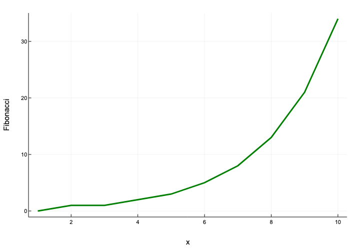
begin
    plot(sequence, xlabel="x", ylabel="Fibonacci", linewidth=3, label=false, color="green", size=(450, 300))
    scatter!(sequence, label=false, color="purple", size=(450, 300))
end
In the example above, a plot is created when we call the plot() function.
What the scatter!() call then does, is to modify the global state of the plot in-place.
If not done this way, both plots wouldn’t be sketched together.
A nice feature that the Plots.jl package offers, is the fact of changing plotting backends.
There exist various plotting packages in Julia, and each one has its own special features and aesthetic flavour.
The Plots.jl package integrates these plotting libraries and acts as an interface to communicate with them in an easy way.
By default, the GR backend is the one used.
In fact, this was the plotting engine that generated the plots we have already done.
The most used and maintained plotting backends up to date, are the already mentioned GR, Plotly/PlotlyJS, PyPlot, UnicodePlots and InspectDR.
The backend you choose will depend on the particular situation you are facing.
For a detailed explanation on backends, we recommend you visit the Julia Plots documentation.
Through the book we will be focusing on the GRbackend, but as a demonstration of the ease of changing from one backend to another, consider the code below.
The only thing added to the code for plotting that we have already used, is the pyplot() call to change the backend.
If you have already coded in Python, you will feel familiar with this plotting backend.
begin
    pyplot()
    plot(sequence, xlabel="x", ylabel="Fibonacci", linewidth=3, label=false, color="green", size=(450, 300))
    scatter!(sequence, label=false, color="purple", size=(450, 300))
end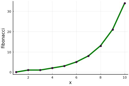
Analogously, we can use the plotlyjs backend, which is specially suited for interactivity.
begin
    plotlyjs()
    plot(sequence, xlabel="x", ylabel="Fibonacci", linewidth=3, label=false, color="green", size=(450, 300))
    scatter!(sequence, label=false, color="purple", size=(450, 300))
end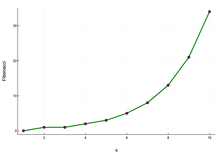
Each of these backends has its own scope, so there may be plots that one backend can do that other can’t. For example, 3D plots are not supported for all backends. The details are well explained in the Julia documentation. "
2.5.2 Introducing DataFrames.jl
When dealing with any type of data in large quantities, it is essential to have a framework to organize and manipulate it in an efficient way. If you have previously used Python, you probably came across the Pandas package and dataframes. In Julia, the DataFrames.jl package follows the same idea. Dataframes are objects with the purpose of structuring tabular data in a smart way. You can think of them as a table, a matrix or a spreadsheet. In the dataframe convention, each row is an observation of a vector-type variable, and each column is the complete set of values of a given variable, across all observations. In other words, for a single row, each column represents a realization of a variable. Let’s see how to construct and load data into a dataframe. There are many ways you can accomplish this. Consider we had some data in a matrix and we want to organize it in a dataframe. First, we are going to create some ‘fake data’ and loading that in a Julia DataFrame,
begin
    using DataFrames, Random

    Random.seed!(123)

    fake_data = rand(5, 5) # this creates a 5x5 matrix with random values between 0
                           # and 1 in each matrix element.

    df = DataFrame(fake_data)
end
## 5×5 DataFrame
## Row │ x1 x2 x3 x4 x5
## │ Float64 Float64 Float64 Float64 Float64
## ─────┼───────────────────────────────────────────────────
## 1 │ 0.768448 0.662555 0.163666 0.463847 0.70586
## 2 │ 0.940515 0.586022 0.473017 0.275819 0.291978
## 3 │ 0.673959 0.0521332 0.865412 0.446568 0.281066
## 4 │ 0.395453 0.26864 0.617492 0.582318 0.792931
## 5 │ 0.313244 0.108871 0.285698 0.255981 0.20923As you can see, the column names were initialized with values \(x1, x2, ...\).
We probably would want to rename them with more meaningful names.
To do this, we have the rename!() function.
Remember that this function has a bang, so it changes the dataframe in-place, be careful!
Below we rename the columns of our dataframe,
rename!(df, ["one", "two", "three", "four", "five"])## 5×5 DataFrame
## Row │ one two three four five
## │ Float64 Float64 Float64 Float64 Float64
## ─────┼───────────────────────────────────────────────────
## 1 │ 0.768448 0.662555 0.163666 0.463847 0.70586
## 2 │ 0.940515 0.586022 0.473017 0.275819 0.291978
## 3 │ 0.673959 0.0521332 0.865412 0.446568 0.281066
## 4 │ 0.395453 0.26864 0.617492 0.582318 0.792931
## 5 │ 0.313244 0.108871 0.285698 0.255981 0.20923The first argument of the function is the dataframe we want to modify, and the second an array of strings, each one corresponding to the name of each column. Another way to create a dataframe is by passing a list of variables that store arrays or any collection of data. For example, "
DataFrame(column1=1:10, column2=2:2:20, column3=3:3:30)## 10×3 DataFrame
## Row │ column1 column2 column3
## │ Int64 Int64 Int64
## ─────┼───────────────────────────
## 1 │ 1 2 3
## 2 │ 2 4 6
## 3 │ 3 6 9
## 4 │ 4 8 12
## 5 │ 5 10 15
## 6 │ 6 12 18
## 7 │ 7 14 21
## 8 │ 8 16 24
## 9 │ 9 18 27
## 10 │ 10 20 30As you can see, the name of each array is automatically assigned to the columns of the dataframe. Furthermore, you can initialize an empty dataframe and start adding data later if you want,
begin
    df_ = DataFrame(Names = String[],
                Countries = String[],
                Ages = Int64[])
    df_ = vcat(df_, DataFrame(Names="Juan", Countries="Argentina", Ages=28))
end
## 1×3 DataFrame
## Row │ Names Countries Ages
## │ String String Int64
## ─────┼──────────────────────────
## 1 │ Juan Argentina 28We have used the vcat()function seen earlier to append new data to the dataframe.
You can also add a new column very easily,
begin
    df_.height = [1.72]
    df_
end
## 1×4 DataFrame
## Row │ Names Countries Ages height
## │ String String Int64 Float64
## ─────┼───────────────────────────────────
## 1 │ Juan Argentina 28 1.72You can access data in a dataframe in various ways. One way is by the column name. For example,
df.three## 5-element Array{Float64,1}:
## 0.16366581948600145
## 0.4730168160953825
## 0.8654121434083455
## 0.617491887982287
## 0.2856979003853177df."three"## 5-element Array{Float64,1}:
## 0.16366581948600145
## 0.4730168160953825
## 0.8654121434083455
## 0.617491887982287
## 0.2856979003853177But you can also access dataframe data as if it were a matrix. You can treat columns either as their column number or by their name,
df[1,:]## DataFrameRow
## Row │ one two three four five
## │ Float64 Float64 Float64 Float64 Float64
## ─────┼─────────────────────────────────────────────────
## 1 │ 0.768448 0.662555 0.163666 0.463847 0.70586df[1:2, "one"]## 2-element Array{Float64,1}:
## 0.7684476751965699
## 0.940515000715187df[3:5, ["two", "four", "five"]]## 3×3 DataFrame
## Row │ two four five
## │ Float64 Float64 Float64
## ─────┼───────────────────────────────
## 1 │ 0.0521332 0.446568 0.281066
## 2 │ 0.26864 0.582318 0.792931
## 3 │ 0.108871 0.255981 0.20923The column names can be accessed by the names() function,
names(df)## 5-element Array{String,1}:
## "one"
## "two"
## "three"
## "four"
## "five"Another useful tool for having a quick overview of the dataframe, typically when in an exploratory process, is the describe() function.
It outputs some information about each column, as you can see below,
describe(df)## 5×7 DataFrame
## Row │ variable mean min median max nmissing eltype
## │ Symbol Float64 Float64 Float64 Float64 Int64 DataType
## ─────┼───────────────────────────────────────────────────────────────────────
## 1 │ one 0.618324 0.313244 0.673959 0.940515 0 Float64
## 2 │ two 0.335644 0.0521332 0.26864 0.662555 0 Float64
## 3 │ three 0.481057 0.163666 0.473017 0.865412 0 Float64
## 4 │ four 0.404907 0.255981 0.446568 0.582318 0 Float64
## 5 │ five 0.456213 0.20923 0.291978 0.792931 0 Float64To select data following certain conditions, you can use the filter() function.
Given some condition, this function will throw away all the rows that don’t evaluate the condition to true.
This condition is expressed as an anonymous function and it is written in the first argument.
In the second argument of the function, the dataframe where to apply the filtering is indicated.
In the example below, all the rows that have their ‘one’ column value greater than \(0.5\) are filtered.
filter(col -> col[1] < 0.5, df)## 2×5 DataFrame
## Row │ one two three four five
## │ Float64 Float64 Float64 Float64 Float64
## ─────┼──────────────────────────────────────────────────
## 1 │ 0.395453 0.26864 0.617492 0.582318 0.792931
## 2 │ 0.313244 0.108871 0.285698 0.255981 0.20923A very usual application of dataframes is when dealing with CSV data. In case you are new to the term, CSV stands for Comma Separated Values. As the name indicates, these are files where each line is a data record, composed by values separated by commas. In essence, a way to store tabular data. A lot of the datasets around the internet are available in this format, and naturally, the DataFrame.jl package is well integrated with it. As an example, consider the popular Iris flower dataset. This dataset consists of samples of three different species of plants. The samples correspond to four measured features of the flowers: length and width of the sepals and petals. To work with CSV files, the package CSV.jl is your best choice in Julia. Loading a CSV file is very easy once you have it downloaded. Consider the following code,
begin
    using CSV

    iris_df = CSV.File("./02_julia_intro/data/Iris.csv") |> DataFrame
end
## 150×6 DataFrame
## Row │ Id SepalLengthCm SepalWidthCm PetalLengthCm PetalWidthCm Specie ⋯
## │ Int64 Float64 Float64 Float64 Float64 String ⋯
## ─────┼──────────────────────────────────────────────────────────────────────────
## 1 │ 1 5.1 3.5 1.4 0.2 Iris-s ⋯
## 2 │ 2 4.9 3.0 1.4 0.2 Iris-s
## 3 │ 3 4.7 3.2 1.3 0.2 Iris-s
## 4 │ 4 4.6 3.1 1.5 0.2 Iris-s
## 5 │ 5 5.0 3.6 1.4 0.2 Iris-s ⋯
## 6 │ 6 5.4 3.9 1.7 0.4 Iris-s
## 7 │ 7 4.6 3.4 1.4 0.3 Iris-s
## 8 │ 8 5.0 3.4 1.5 0.2 Iris-s
## ⋮ │ ⋮ ⋮ ⋮ ⋮ ⋮ ⋱
## 144 │ 144 6.8 3.2 5.9 2.3 Iris-v ⋯
## 145 │ 145 6.7 3.3 5.7 2.5 Iris-v
## 146 │ 146 6.7 3.0 5.2 2.3 Iris-v
## 147 │ 147 6.3 2.5 5.0 1.9 Iris-v
## 148 │ 148 6.5 3.0 5.2 2.0 Iris-v ⋯
## 149 │ 149 6.2 3.4 5.4 2.3 Iris-v
## 150 │ 150 5.9 3.0 5.1 1.8 Iris-v
## 1 column and 135 rows omittedHere we used the pipeline operator |>, which is mainly some Julia syntactic sugar.
It resembles the flow of information.
First, the CSV.File()function, loads the CSV file and creates a CSV File object, that is passed to the DataFrame()function, to give us finally a dataframe.
Once you have worked on the dataframe cleaning data or modifying it, you can write a CSV text file from it and in this way, you can share your work with other people.
For example, consider I want to filter one of the species of plants, ‘Iris-setosa,’ and then I want to write a file with this modified data to share it with someone,
begin
    filter!(row -> row.Species != "Iris-setosa", iris_df)
    CSV.write("./02_julia_intro/data/modified_iris.csv", iris_df)
end;
Plotting Dataframes data is very easy.
Suppose we want to plot the flower features from the iris dataset, all in one single plot.
These features correspond to the columns two to five of the dataframe.
Thinking about it as a matrix, you can access these data by selecting all the rows for each of the corresponding columns.
In the code below, a loop is performed over the columns of interest.
The plot() statement, with no arguments, is a way to create an empty instance of a plot, like a blank canvas.
This empty plot will be successively overwritten by each call to plot!().
Finally, we make a call to current(), to display the plot.
You may be wondering why this is necessary.
Notice that all the plotting happens inside a loop, hence the plotting iterations are not displayed.
It is more efficient to display the finished plot when the loop is over than to update each plot as it overwrites the previous one.
begin
    gr()
    plot()
    for i in 2:5
        plot!(iris_df[:,i], legend=false)
    end
    xlabel!("Flower")
    ylabel!("Centimeters (cm)")
    title!("Flower features")
    current()
end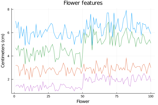
2.6 Summary
In this chapter we have introduced the Julia language, the motivations behind its creation, features, installation and basic building blocks for writing some code. First we discussed some basic Julia operators and datatypes. Some special features of the language such as how to write different kinds of arrays and broadcasting were detailed. We then followed with an overview of how functions work in Julia, and how to make your own. Finally, we introduced some packages of the Julia ecosystem, mainly the Plots.jl package for plotting and changing backends, and DataFrames.jl for data organization and manipulation.